Interpreting NDVI: Uses, Context, and Limitations

Understand the index before interpreting its colors

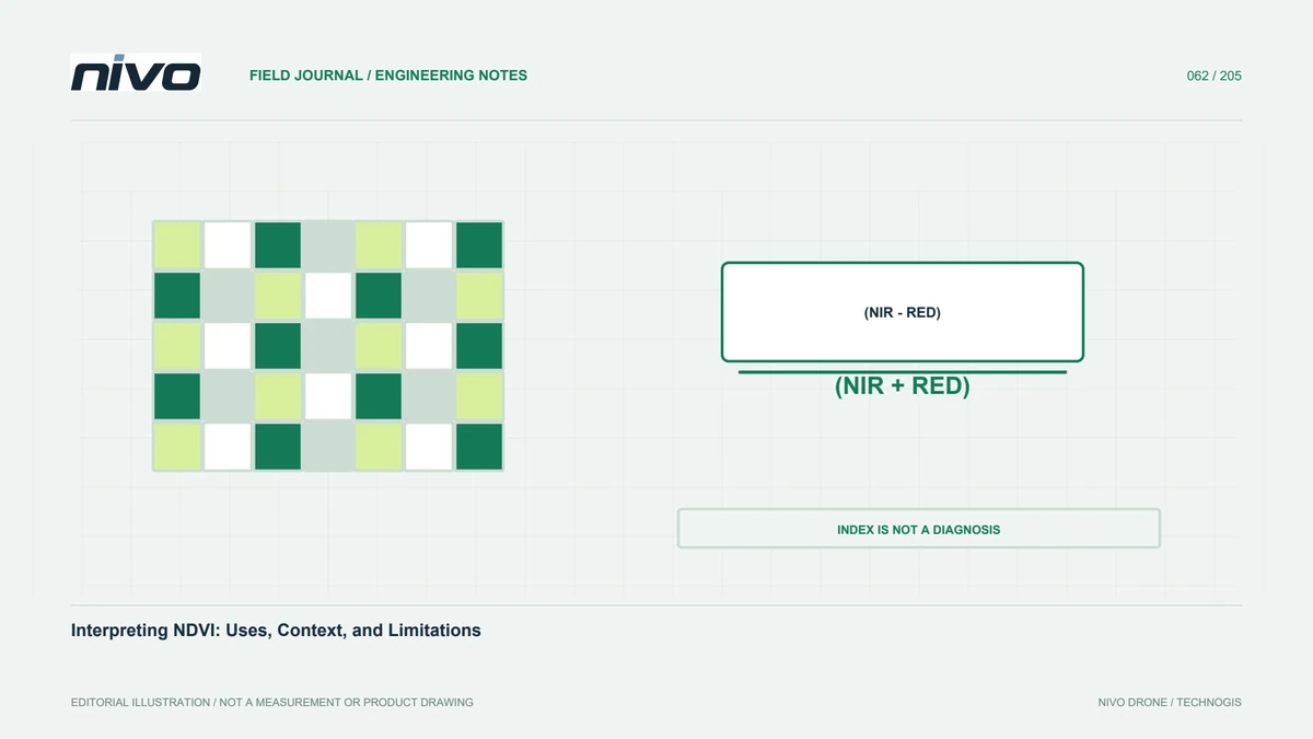
NDVI uses the relationship between red and near-infrared reflectance to describe vegetation greenness. It does not independently identify the cause of every pattern. Map colors represent numbers, not diagnoses. Before interpretation, review the channels, processing method, and legend definition. Similar colors on two maps can represent different ranges, while different colors can represent the same value under a changed palette. Checking values and context prevents the simplistic assumption that the greenest displayed area must always have the best crop condition.

Relate values to cover and growth stage

A pixel can contain leaves, soil, shadow, water, or mixtures. In young crops, exposed soil between rows can strongly influence the observed pattern. Relationships can change as the canopy closes. Record age, crop type, planting pattern, and cover before comparing parcels. Do not transfer an interpretation from one growth stage automatically to another. A field with lower cover may simply have been planted later. Meaningful interpretation needs the spectral response connected to known management circumstances rather than a presumed universal scale of crop health.

Check the inputs that produced the index

A mathematically correct index can mislead when its input images are unsuitable. Review band alignment, corrections, exposure, and metadata completeness. Misaligned channels can create sharp artifacts by combining different objects. Inconsistent lighting or calibration can also influence comparison. Inspect source images wherever the index appears unusual. Do not erase a pattern as noise without investigating its origin. Read quality notes with the map to separate areas suitable for interpretation from those needing review or recapture before decisions rely on the displayed values.

Do not transfer thresholds without testing

A threshold useful on one farm may mean something different elsewhere because crops, age, soils, water, sensors, or processing differ. Explain whether classes are relative within one dataset or based on validated boundaries. Relative classes can help locate unusual areas without acting as universal health categories. Validate intended management thresholds through field observations. Preserve the rationale and supporting examples so that later decisions can be reviewed. A clearly stated classification method is more useful than presenting familiar colors as if their meaning were self-evident.

Use spatial patterns to build hypotheses

Pattern shape can guide field questions. Variation following crop rows may suggest a different investigation from variation following drainage or management boundaries. Treat these relationships as hypotheses rather than confirmed causes. Compare indices with parcel maps, activity histories, and available terrain information. Select examples of the main patterns and suitable comparison areas. The map narrows the investigation without replacing direct observation. Record unexplained patterns as potential information gaps, because they can reveal what supporting data or redesigned acquisition the next survey should include.

Design field checks without selection bias

Visiting only low-value areas can overlook normal variation elsewhere. Sample several classes, including apparently good areas and pattern boundaries. Use consistent location identities to connect findings to pixels or zones. Record dates, crop condition, soil cover, water, and relevant management information. Separate observed facts from suspected explanations. Involve agronomic expertise where additional measurements are needed. Good comparison observations may overturn the initial interpretation, showing, for example, that age differences explain a pattern better than the disturbance first suspected from the map alone.

Compare dates with methods in view

Repeated monitoring needs more than the same index formula. Examine sensor, calibration, illumination, crop stage, area boundaries, and processing comparability. Mark method changes rather than treating them as biological change. If colors are automatically rescaled, provide a comparison view with explicit values. More red after a legend change is not proof of deterioration. State meaningful differences in observation conditions and how they limit the question being answered. Specific comparison boundaries make the time series more useful than an apparently precise change map with unexplained assumptions.

Translate observations into staged decisions

Separate what was observed, how it is interpreted, and what action should follow. A differing-value zone is an observation; a relationship to field findings is an interpretation; a visit or further measurement is a possible next step. Do not turn one NDVI map into an application prescription that bypasses agronomic assessment. Show the evidence and unresolved questions behind each recommendation. This helps recipients understand how imagery contributes to the decision and makes the map part of a documented learning process rather than an unexplained colored deliverable.

Retain an analytical audit trail

Archive source images, index parameters, legends, field boundaries, calibration records, and ground observations together. Record when and where management actions occur so later observations have context. Evaluate whether priority zones genuinely help identify relevant conditions. If they do not, revisit sampling, acquisition, or index choice. NDVI is valuable when used for suitable questions with supporting evidence. Its practical strength comes from traceable relationships between spectral response, actual conditions, and management choices, not from assuming one number summarizes every aspect of plant health.

Illustrative case: a changed legend that looks like crop deterioration

Imagine a hypothetical manager comparing two NDVI maps on a screen. The later map contains more red areas, so the immediate conclusion is that crop condition has deteriorated across the farm. Before accepting that interpretation, the analyst checks the numerical legends and discovers that each map was styled independently using its own value distribution. A red pixel on one date therefore does not necessarily represent the same index value as a red pixel on the other. The team retains both original presentations but creates a comparison view with explicit, consistent class definitions.

The analyst then reviews calibration, growth stage, boundaries, and geometric alignment rather than assuming that a corrected legend resolves every comparison issue. Several field-check locations are selected from apparent decreases, stable areas, and boundary zones. Observations distinguish what was seen from suspected explanations. The final note shows numerical changes alongside the conditions that can affect their meaning and identifies questions requiring agronomic assessment. Any recommendation is linked to supporting evidence rather than to a color alone. This hypothetical case demonstrates how presentation choices can create a persuasive change narrative and why interpreting an index requires values, methods, and field context to remain visible throughout the decision process.

The handover contrasts two statements: the map now uses a fair comparison legend, and the evidence demonstrates a crop change. Only the first follows directly from restyling. The second still needs appropriate acquisition, processing, and field support. The reviewer receives both original legends, the common classification definition, numerical summaries, and locations selected for checking. Acceptance means those records can explain the finding without relying on color impressions. This protects a genuine change signal from being dismissed while also preventing presentation differences from being promoted into unsupported biological conclusions.